Forward looking vs backward looking return forecasts
Trying to forecast short term returns has always been quite a difficult task for asset allocators and investors in general, however the “textbook” method to forecast returns is an old, backward-looking phenomenon, which can certainly be improved on by incorporating simple, forward-looking metrics. Traditional portfolio management textbooks teach you “mean-variance optimization” which has its own set of flaws and one of the inputs to that optimization is what we’ll talk about today, expected returns (others being expected risk /covariance matrix). These “expected returns” dictate the return outlook for a particular asset class and are a vital component of asset allocation – we will not touch on expected risk in this piece.
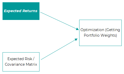
“Classic, Textbook example”
The classic example is what’s known as the “constant expected return” (CER) model. It assumes that an asset’s return and risk are constant or what we call “time-invariant”. It uses the “average monthly return” as the input, assuming the future returns of that asset will look like the long-term average monthly return. Whilst this model does face its flaws, it is a useful benchmark against more complex models, such as the forward-looking model we will see below. When we say “forward-looking”, we refer to using information today that is available, that informs return outcomes of an asset in the future. By contrast, the CER simply just assumes the future return of an asset is equal to what it has returned as far back as the data goes – which in itself may cause inhibiting biases.
“Forward-looking” model
This specific model has 2 components to it: 1) Mean Reversion (Valuation), 2) Momentum, defined as 5-year cumulative return and 12-month cumulative return respectively. What we’re essentially asking ourselves today is, what was the past 5-year cumulative return and 12-month cumulative return of a particular asset and does that have an effect on the future returns of that asset (in this example we look at 12-month forward returns). Our research, and several other pieces of academic literature point to a relationship between the future 12-month returns and these 2 factors. What we’re essentially saying is that the next 12-month returns are a function of the previous 5y returns and the previous 12-month returns – so, why not model it?
Mean Reversion
The intuition for mean-reversion is that asset returns tend to revert to some long-term average, which is in the name. Given this, intuitively, it makes sense that there would be a negative relationship between the 5y cumulative return of an asset and the future 12-month return. Meaning, if an asset has performed very well for the past 5-years, we expected that asset to not do as well as an asset that has performed very poorly over the past 5-years. This factor may also be referred to as “valuation”. Asness, Moskowitz, and Pedersen (2013), Greenwood, Shleifer, and You (2017), have similarly used 5-year return as a proxy for valuation prediction for future expected return. As Rozeff (1984), Fama and French (1988), and many others have studied, valuations drive expected returns.
Momentum
The intuition behind momentum is less obvious, but is primarily attributed to “behavioral” explanations, such as investor herding and underreaction (overreaction) to positive (negative) news for an asset which in turn leads to delayed “momentum” for the asset. This phenomenon has been very well documented in the academic literature and was added onto the Fama French 3 Factor model (1993) as a part of the Carhart 4 Factor model (1997) to further increase the explain ability of the cross-section of stock returns and fund manager performance (Initially brought to the academic world by Jegadeesh and Titman (1993)). Time series momentum is significant across all asset classes, as studied by Moskowitz, Ooi and Pedersen (2011). A common finding is also the reversals following these momentum anomalies, where those assets with strong 12m momentum tend to experience abnormal negative returns 12 months after the formation date, and dissolve after 2 years. Overall, the literature and research suggest that avoiding assets that have been falling for the past 12-months and buying those that have been rising for the past 12-months proves value-accretive.
Method & Results
Here, we will run a simple comparison between these 2 types of models, and further, simulate portfolios that buy assets based on the “expected return” outputs these models put forward. Everything else will be held constant, e.g., both will use the sample covariance matrix and a simple mean-variance optimization each month, with an expanding window on expected returns and the covariance matrix, with 12-years as the initial in-sample “window” to establish parameters. Doing so allows for an out of sample walk-forward optimization after that 12-year window each month.
Note: I restrict the portfolio turnover to only 1/12th of the portfolio each month (given we forecast 12-month forward), to make for a more practical example.
The 5 assets used for this back test were:
- US equities
- US Bond Aggregate
- Japanese equities
- German equities
- Commodities Index
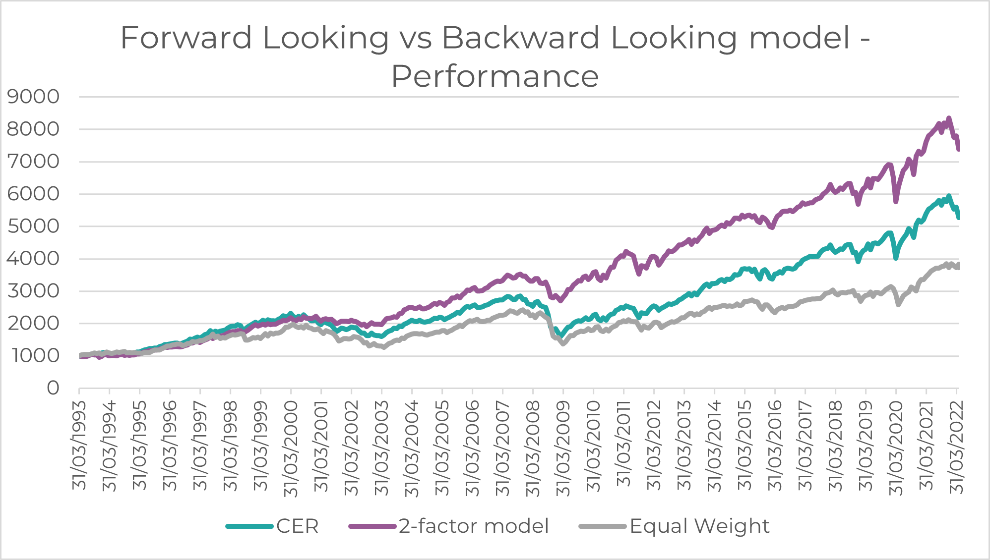
Source: Innova Asset Management, Bloomberg
As seen above, and in the table below, the 2-factor model significantly reduces drawdowns, volatility and is able to harvest more returns given its forward-looking nature. We use a naïve “equal-weighted” benchmark too, which is a simple equal-weight of all 5 assets.

This back-test proves the efficacy and effectiveness of a forward-looking model, which highlights that 12-month forward returns are a function of 12-month cumulative returns, and 5y cumulative returns. By moving beyond a static assumption of expected returns (CER model), the 2-factor model is able to re-weight the allocation to bonds, equities and commodities, based on their current ex-ante level of expected returns.
Dynamism during drawdowns - GFC
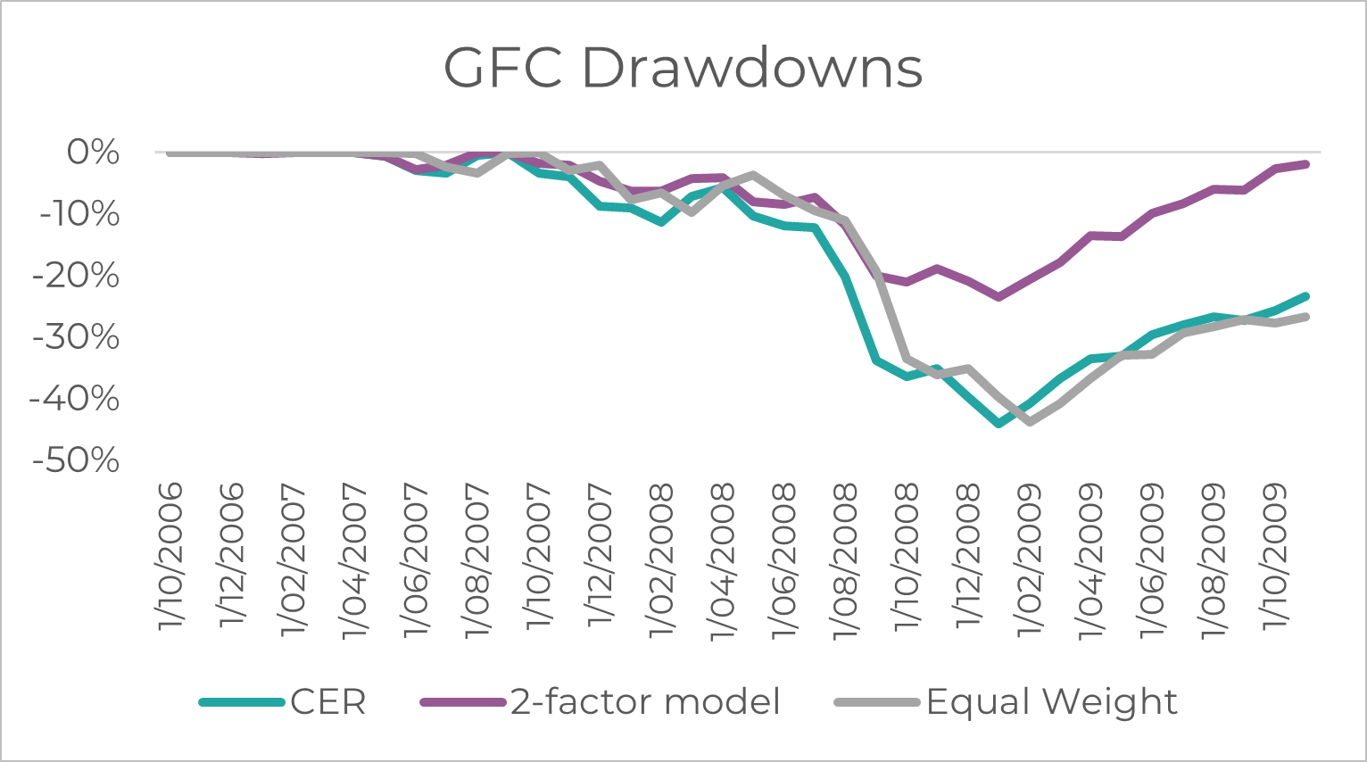
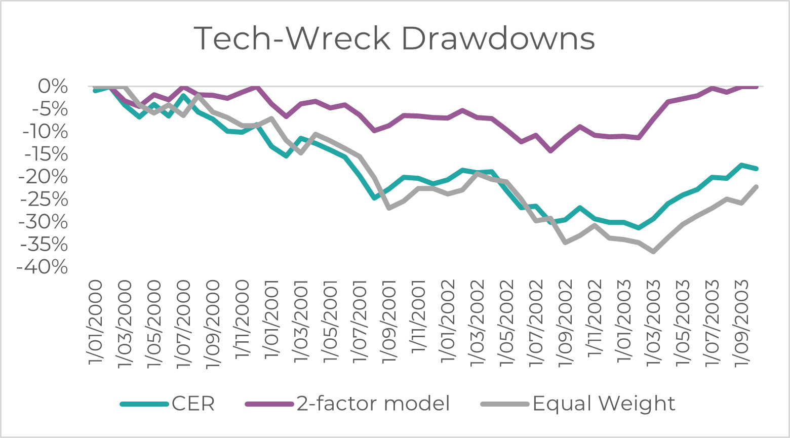
Below, we can clearly see the value-add of including factors such as mean-reversion and momentum into your expected return framework during a recession / harsh drawdown. Right before the recession, the mean-reversion component plays a significant role in mitigating risk by lowering the weight in assets with stretched valuation levels. Before a recession you generally get heightened valuations on risk assets, which causes the harsher drawdowns for the CER model, having only a ~20% allocation to US bonds. The 2-factor model on the other hand reached an almost ~80% bond (duration) allocation, limiting the steepness of drawdown.
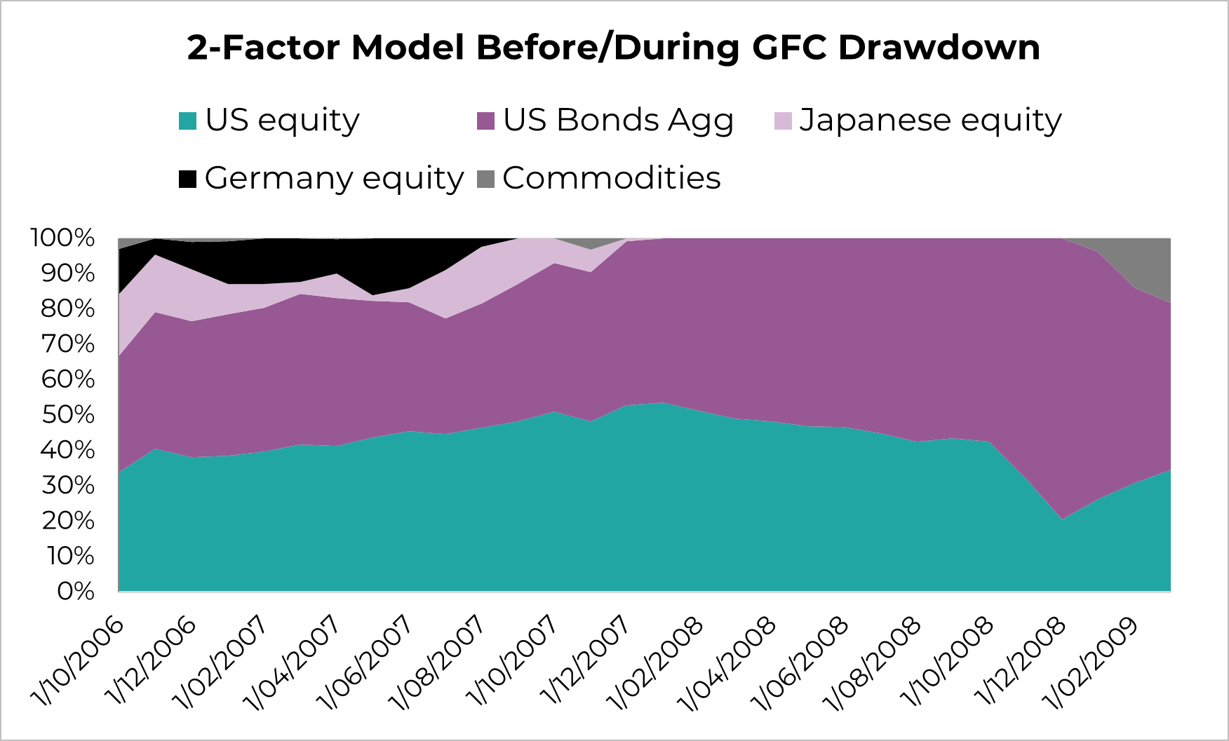
Source: Innova Asset Management, Bloomberg
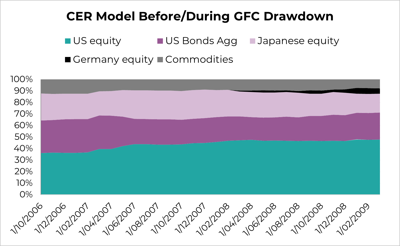
As seen below, not only do we get more resilient portfolios in the 2 major drawdowns, but also a significantly quicker recovery, and therefore capital preservation for investors.
Source: Innova Asset Management, Bloomberg
Source: Innova Asset Management, Bloomberg
Considering forward looking factors is just a way of improving one of the building blocks involved in the overall asset allocation / portfolio construction process – expected returns. Momentum and mean-reversion also have very intuitive economic reasoning and allow for multi-asset allocators to build more forward-looking, risk-aware portfolios.
References
Asness, C. S., Moskowitz, T. J., & Pedersen, L. H. (2013). Value and momentum everywhere. The journal of finance, 68(3), 929-985.
Carhart, M. M. (1997). On persistence in mutual fund performance. The Journal of finance, 52(1), 57-82.
Fama, E. F., & French, K. R. (1988). Permanent and temporary components of stock prices. Journal of political Economy, 96(2), 246-273.
Fama, E. F., & French, K. R. (1993). Common risk factors in the returns on stocks and bonds. Journal of financial economics, 33(1), 3-56.
Greenwood, R., Shleifer, A., & You, Y. (2017). Bubbles for Fama, No. 23191.
Jegadeesh, N., & Titman, S. (1993). Returns to buying winners and selling losers: Implications for stock market efficiency. The Journal of finance, 48(1), 65-91.
Moskowitz, T. J., Ooi, Y. H., & Pedersen, L. H. (2012). Time series momentum. Journal of financial economics, 104(2), 228-250.
Rozeff, M. S. (1984). Dividend yields are equity risk premiums. Journal of Portfolio management, 68-75.
5 topics

